

The fundamental tools of operations science (also called decision science) were designed with factories and warehouses in mind. But they are easily applicable to video game art asset pipelines. In this post, I’ll walk you through the basics of how operation science looks at pipelines, called “process flows” in operations speak.
The article image for “Video Game Art Pipelines” is from GraphicStock. Used under license.
By Reading This Post, You’ll Learn:
- How to use process flow charts to estimate the time necessary to complete an asset
- The formal definition of bottlenecks and critical paths
- Little’s Law and how to use it to infer information about pipelines
- How to calculate the iceiciency level of your pipelines
- How to identify opportunities to improve process flows and how to go about improving them
The Basics of Video Game Art Asset Pipelines
Consider a hypothetical production pipeline. This pipeline could be fore anything. Building cars, fulfilling Amazon orders, or creating video game art assets. Assume every activity in this pipeline is required to turn inputs into outputs, and each activity can only handle one unit at a time. The the total number of units that are in the pipeline somewhere between input and output is called the in-process inventory (I).
You’ll notice that the pipeline branches at Activity B before reforming at Activity G.

A basic process flow diagram, with a branching path.
Critical Path = Theoretical Flow Time
The upper path takes longer than the lower branch, making it the critical path from input to output. The activities on that path are called the critical activities:

The longest path from input to output (highlighted in red) is called the “critical path”
The critical path determines the minimum time required to take an asset from input to output. The sum of all the activities on the Critical Path (A, B, C, D, E, and G) is 13 hours. The fastest a unit will go from input (eg, raw materials) to output (finished car) is 13 hours.
In Operation Science terms, your Critical Path determines your theoretical flow time (TFT). TFT is the shortest possible flow time, under ideal conditions. So, no mistakes and nobody ever needs to take a bathroom break. Further, units instantaneously transition from on process to the next with zero downtime.
You can also calculate the theoretical flow time of any section of the pipeline or individual activities. The theoretical flow time to get from input to the start of Activity C is 3 hours. The theoretical flow time of Activity E is 5 hours.
Bottleneck = Throughput
Meanwhile, Activity F is the bottleneck – it is the single longest activity of the entire pipeline:

The single longest activity (highlighted in red) is called “the bottleneck”
More specifically, the bottleneck has the lowest throughput (R), or average rate of processing units. In our hypothetical pipeline, the bottleneck requires 8 hours to complete. The entire process will output one unit every 8 hours or 1/8 of a unit every hour (more on that further down). The bottleneck does not need to lie on the critical path. It is simply the longest single activity.
The throughput of the bottleneck determines the throughput of the entire pipeline. Therefor, your pipeline will never produce units with a faster periodicity than your bottleneck.
You can base your throughput on whatever unit of time makes the most sense (seconds, hours, days, months, etc). You can also define a “unit” as the denomination that makes the most sense (1 character model, a dozen doughnuts, a gallon of wine, 500 lbs of novelty rubber dog poo, etc).
But There’s More to Throughput than Just the Time Per Activity
Like flow time, you can calculate throughput at a per-activity level. For example, Activity A takes half the time of Activity B and thus has twice the throughput for any given unit of time.
Finally, throughput is based not just on the length of time an activity takes, but by the number of resources performing that activity. If rigging a character model takes 8 hours, but you have 2 artists doing the rigging, then your throughput is 2 models every 8 hours, or an average of 1 model every 4 hours.
By extension, this means that by adding resources to a pipeline, you can effectively change which activity has the lowest average output and is thus the bottleneck. I cover this topic in more detail in Part 2. For now, keep things simple and assume each activity has a single resource.
Calculating Your Actual Flow Time Using Little’s Law
In addition to TFT, you need to calculate your average wait time. Wait time is the time a unit spends waiting for the next activity to start of for an interrupted process to resume. In short, wait time is the time the unit spends not doing anything.
When your concept artist finishes her full color character design of Master Chief and hands it off to your character modeler, that hand-off time is wait time. If the modeler needs to finish his current high-poly model before he can sculpt Master Chief , that queue time is also Wait Time. When the modeler goes home for the day with a half-finished Master Chief model, that also is wait time.
If you know your TFT and wait time, you can add them together to calculate your actual process flow time (T): TFT + wait time = T. T is the average time it takes for units to actually move through the pipeline.
Again, TFT is the ideal time to move one unit through the entire pipeline, with zero waiting. T is the time the process takes in the real world. The beauty of this equation’s simplicity is that you can also back into your wait time (and thus analyze your efficiency) if you could somehow calculate your average process flow time directly.
Enter Little’s Law. In a steady-state process (eg, inventory is entering the system at the same average rate it leaves), inventory is equal to your process flow time multiplied by your throughput. Or, more simply: I = RT.
An Example of Little’s Law from Literature
Remember that scene in Aliens where Ripley suddenly realizes that she and Newt have stumbled into the queen’s chamber? And you get that long, really horrifying, nauseating close-up of the egg-sack?
Well, let’s assume that the egg-sack has a throughput of 5 eggs every day on average:

Next, lets assume that her process flow time is 7 days for a single egg to go from genesis (or whatever happens in there) to being deposited on the hive floor:

Finally, let’s make one final assumption that the queen starts creating new eggs at the same rate she deposits them (again, on average). The average in-process inventory of eggs within the sack is 5*7 = 35 eggs.
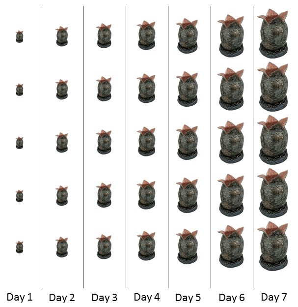 If it takes 7 days to create an egg, in order to produce a 5-egg-per-day throughput, 35 eggs have to be in the sack on average. There is simply no other way that the queen could sustain that average throughput, given the lead time produce a new egg.
But, what if you didn’t know the gestation period, but instead knew the inventory in the sack and the throughput? Little’s Law still holds. Take the 35 eggs in the sack, divide by the throughput, 5, and you have the flow time for the queen to produce a single egg. I/R = T, or in this case 35/5 = 7. And Little’s Law holds for figuring out throughput as well: R = I/T
Applying Little’s Law To Your Pipeline
To determine your average process flow time of the entire pipeline, first identify the theoretical flow time (or the actual flow time, if you know it) of the bottleneck. In the chart above, the TFT of the bottleneck is 8 hours. The inverse of that number is the throughput (R = 1/TFT)* of the entire pipeline.
In the example above, assuming an 8-hour day, the bottleneck (and thus the entire process) will produce 1/8 of a unit per hour, 1 unit per day, and 5 units per week, depending on what time unit you want to use.
Now inventory every asset currently in some state of progress in the pipeline. Ignore assets on your backlog that you haven’t started and assets that are compete. Divide that inventory by the throughput you calculated above and the result is your process flow time.
Resources That Informed And Influenced This Post
If you have ad blockers turned on, you may not see the above links. Breaking The Wheel is part of Amazon’s Affiliate Program. If you purchase products using the above links, the blog will get a portion of the sale (at no cost to you).
Calculating Flow Time Efficiency
Finally, divide your theoretical flow time by the process flow time, to determine your flow time efficiency: FTE = TFT/T. This is a measurement of how close you are to an ideal pipeline. More specifically, it’s a measurement of how much time your assets spend waiting around for someone to do something with them.
In other words, if your flow time efficiency is 63.7%, your assets spend 36.3% of their time waiting for something to happen.
What can you do with this information? The beauty of Little’s Law (other than it’s simplicity) is you can apply it at any level of granularity. You can apply it to the entire process, some subset of the process, or individual activities.
If you can distinguish between an asset moving through an activity versus assets that are queuing for that activity, you can even apply Little’s Law separately to the queue and the activity.
Improving Your Flow Time Efficiency
If you aren’t happy with your Flow Time Efficiency, break the pipeline down into smaller parts. Then apply Little’s Law to those parts to identify the offending activity or activities. The most likely candidates for a Flow Time Efficiency deficit are:
- Severe mismatches between the throughputs of the various activities in the pipeline, leading to queue build up
- You drastically underestimated the flow time to complete an activity (or inversely, you overestimated the throughput from that activity)
- The team member responsible for the offending activity is barraged with distractions (meetings, other responsibilities, etc) preventing him/her from meeting his/her target throughput
- Or the team member lacks the proper tools to operated at peak performance
- Or the team member is simply not performing up to his/her potential
A Word of Warning About Cracking the Whip
I put number 5 last for a reason. Make sure you have squared away the first four points before you start looking to the individual’s performance. It’s not fair or logical to expect a team member to achieve peak performance if you drag her into four separate one-hour meetings sprinkled throughout the day, breaking up her productive time into small, unconsolidated, inefficient chunks. Nor is it fair or logical to provide her with substandard tools or a PC that crashes once a day and expect her to hit throughput targets.
Unless the team member is blatantly doing something wrong (napping at her desk or arriving late and then leaving early every day), seek first to understand the sources of friction (there are likely several) before you look to the individual’s performance.
Predictability is Virtue All Its Own
Yes cracking the whip can work, but by its nature it’s a short-term strategy, not a sustainable one. You have three high-level goals in operations management: efficiency, sustainability, and predictability. Focus on creating the most efficient environment and process you can. Your ability to do this is constrained by budget and resources. But establishing the maximum level of efficiency you can achieve within your means will create the maximum level of productivity you can sustain long term (ie, without cracking the whip).
If your process is sustainable, it’s predictable. Cracking the whip might yield short term gains, but it’s not sustainable and thus will create volatility in your productivity. This leads to greater variance in your average output. Greater variance means less predictable outcomes, and by extension less reliable schedules. A scheduling errors are a major a major source of crunch.
I’ll go into more detail on variance and its impact in Part 3.
Some Necessary Caveats
It’s important to call out that Little’s Law is a drastic simplification of reality. It provides an average value across all of the units, but tells you nothing of variance. I cover variance in more detail in Part 3.
It also makes a simplifying assumption that the process is in a “steady state”, meaning that the average rate that units enter this system is the same as the average rate at which they exit. If your asset pipelines are anything like the ones I’ve managed, this is probably not going to be the case at any single moment in time. Put simply, you’re going to get a queue build up somewhere in the pipeline.
But this build up probably won’t occur perpetually (ie, you’re not going to accrue an infinite list of work-in-progress assets), so on some level of abstraction (say, the entire course of a project), input = output.
Further Reading If You Enjoyed this Post
Character Art Pipeline Capacity Charts
Video Game Statistics: A Primer
Game Planning With Science! Table of Contents
Little’s Law Holds A Lot of Power For Such A Simple Equation
As far as back-of-the-envelope calculations go, Little’s Law is simple, fast, and flexible. As long as you have any two of the variables, you can calculate the third. In the end, Little’s Law is a diagnostic tool. It won’t solve your problems for you, but it will help you determine where to look.
One Final Note
Little’s Law is also alternatively expressed as L= λW. L is the number of units in the process (same thing as in-process inventory). W is the average time the unit waits in the system (same thing as Flow Time). And λ is the average rate of units arriving into a system which, in a steady-state process, is interchangeable with R (the rate of units leaving the system). In other words, it’s the same formula with different variables and terminology.
Key Takeaways
- Processes, at their most basic level, take inputs and convert them to outputs through a series of activities
- The longest single path from input to output is the Critical Path and the activities on the Critical Path are called Critical Activities
- The longest single activity in the entire process (irrespective of the Critical Path) is the Bottleneck
- The Critical Path determines the Theoretical Flow Time and the Bottleneck determines Throughput
- You actual average process Flow Time is your Theoretical Flow Time + your average Wait Time
- Your flow time efficiency is the measure of how much time your in-process inventory spends waiting for the next activitiy
- In-Process Inventory, Flow Time, and Throughput are all related by Little’s Law – if you know two of them you can calculate the third
Key Equations
- TFT = Theoretical Flow Time
- WT = Average Wait Time
- T = Average Flow Time
- T = TFT + WT
- R = Throughput = 1/T
- I = In-Process Inventory
- I = R*T (Little’s Law)
*This is also an application of Little’s Law. It’s R = I/T with I = 1 because we’re looking for Throughput across a single unit of inventory.
Return to the “Game Planning With Science” Table of Contents

“Video Game Art Pipelines – Game Planning With Science! Part 1” by Justin Fischer is licensed under a Creative Commons Attribution-NonCommercial-ShareAlike 4.0 International License.
Related posts:
 Character Art Pipeline Capacity Charts – Game Planning With Science! Part 2
 Planning Games Using The Central Limit Theorem – Game Planning With Science! Part 4
 User Stories Make For Better Consensus – Game Planning With Science! Part 6
 Scheduling Video Games Scientifically! – Game Planning With Science! Part 7
 Lean Development for Games – Game Planning With Science! Part 9
 GDC17 Feedback and Responses
14 comments
Pingback: Character Art Pipeline Capacity Charts - Game Planning With Science!
Pingback: Poka-Yoke:The Fine Art of Mistake Proofing - Game Planning With Science, Part 10!
Pingback: Kanban: The Counter-Intuitive Value Of Pull-Based Production - Game Planning With Science! Part 11
Pingback: Heijunka: Why Batching Is Not Your Friend - Game Planning With Science, Part 14
Pingback: Make Video Games Scientifically! - Game Planning With Science
Pingback: Lean Development for Games - Game Planning With Science! Part 9
Pingback: Jidoka: Putting The Robots To Work - Game Planning With Science! Part 12
Pingback: Discovery versus Process - An Introduction to Game Planning With Science!
Pingback: The Flawed Logic of Sprints: The Fancy Mess of Scrum, Part 1
Pingback: Conflict of Interest: The Fancy Mess of Scrum, Part 3
Pingback: The Higher Order Consequences of Sprints: The Fancy Mess of Scrum, Part 2
Pingback: User Stories Make for Better Consensus in Feature Estimates